Locator

$$ \mathcal{N}_\Delta : (R,Z) \rightarrow (i_\psi,i_{s\theta},i_{c\theta}) \rightarrow \Delta$$

The mesh generated in the core region is partially ordered, and we can label the triangles using $(i_\psi,i_\theta)$, where $1 \le i_\psi < (m_\psi-1)$ refers to the label of the constant flux contour, with $m_\psi$ number of flux surface, and $i_\theta$ refers to the index of the triangle within each annulus. To find the triangle in which a given point in the poloidal plane lies, we need to find a map \begin{eqnarray} \mathcal{N}_{\Delta} : (R,Z) \rightarrow (i_\psi,i_\theta)\nonumber \end{eqnarray}

\noindent But this map is not smooth, as the index $i_\theta$ has a jump across the outer mid-plane line because of $2\pi$ periodicity. To eliminate the jump we reparametrize the label $i_\theta$ into two variables $i_{c\theta} = \cos(2\pi i_\theta/n_\psi)$, $i_{s\theta} = \sin(2\pi i_\theta/n_\psi)$, where $n_\psi$ is the number of triangles in the annular region. Hence, our goal is to find a smooth function \begin{eqnarray} \tilde{\mathcal{N}}_\Delta : (R,Z) \rightarrow (\tilde{i}_\psi, \tilde{i}_{c\theta}, \tilde{i}_{s\theta})\nonumber \end{eqnarray} such that \begin{eqnarray} i_\psi := \left\lfloor \tilde{i}_\psi \right\rceil \;\;\; \text{and} \;\;\; i_\theta := \left\lfloor \frac{n_\psi}{2\pi} \arctan( \tilde{i}_{s\theta} , \tilde{i}_{c\theta} ) \right\rceil \; , \nonumber \end{eqnarray} where $\left\lfloor . \right\rceil$ refers to the roundoff function.

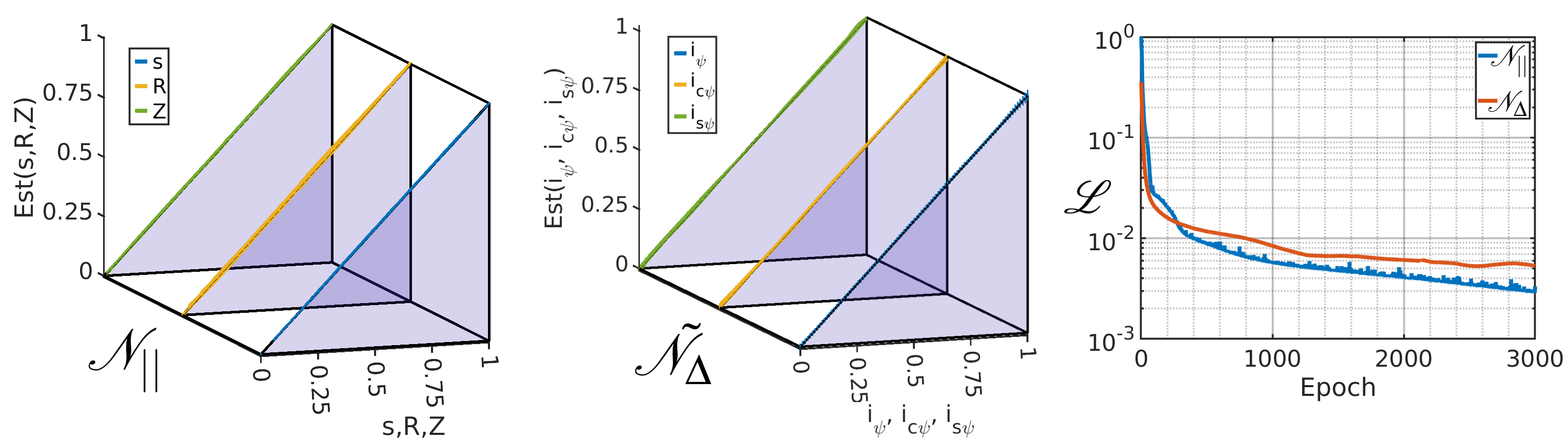
\noindent We use the neural network to estimate the function $\tilde{\mathcal{N}}_\Delta$. The input layer has two nodes, corresponding to $R$ and $Z$, and the output layer has three nodes which correspond to $(\tilde{i}_\psi, \tilde{i}_{c\theta}, \tilde{i}_{s\theta})$. We use ten nodes in the hidden layer with a learning rate of $\eta = 0.001$, and perform training for $\sim 10000$ epochs. The training data is obtained by considering the triangle and the coordinates of the corresponding centroids and tested with randomly distributed points in the mesh. In the next subsection we present the performance of the neural network as $||$-projector and triangle locator.

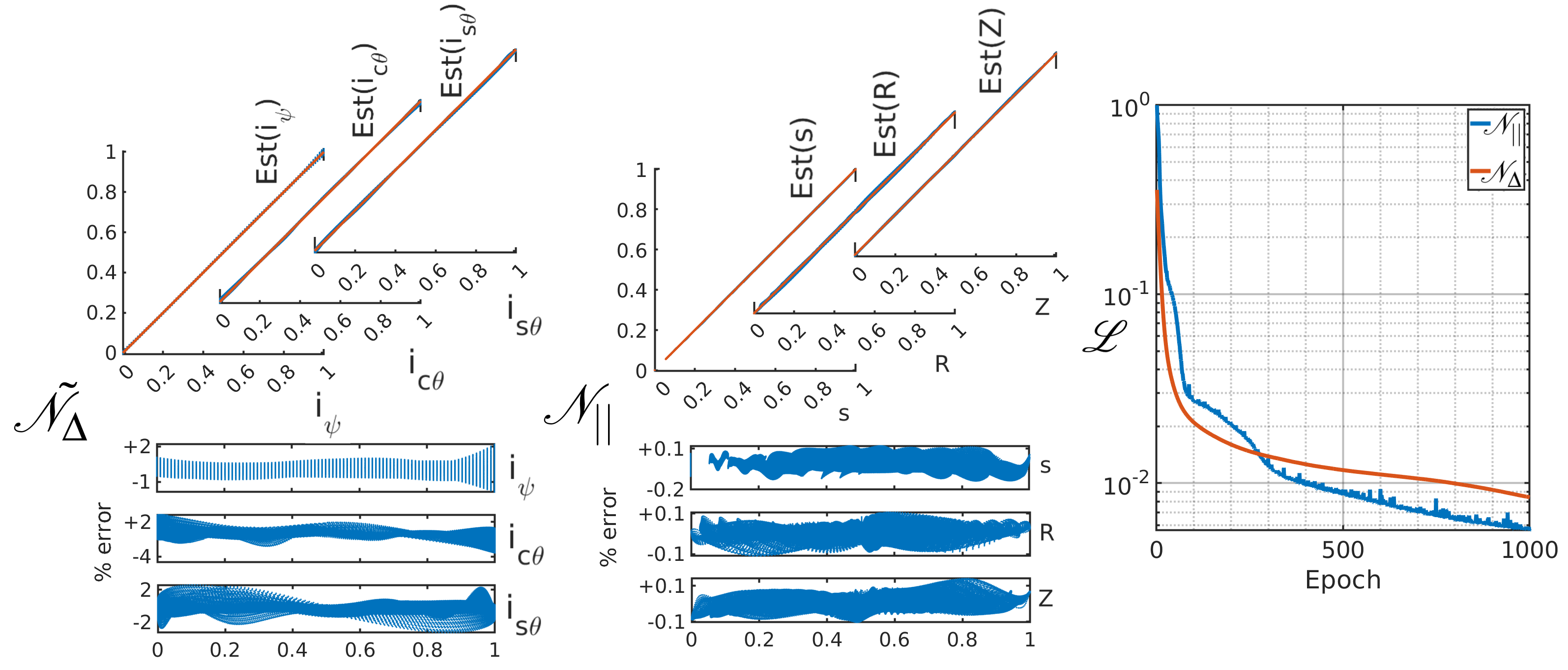
\noindent We visualize the performance of the trained neural network by generating the plot of the predicted value versus the expected value in Fig.(a) and (b) corresponding to the three outputs of $\mathcal{N}_{||}$ and $\tilde{\mathcal{N}}_{\Delta}$. Figure © shows the convergence behaviour of the neural networks using the plot of loss function evolution. In particular, we find that the network can locate the triangle with a maximum error of three to four triangle distances from the correct triangle.

\noindent As indicated in the previous section, the neural network-based triangle locator works well to estimate the triangle in the approximate neighbourhood of the correct triangle. The mesh we use in the simulations is partially structured, so we incorporate an iterative local search scheme to track down the exact triangle in which the particle lies. G2C3 also has a box scheme prescribed in~\cite{Zhixin19} as an alternative to the neural network scheme for locating the triangle, which performs similarly to the neural network approach. For the sake of completeness we describe both the approaches below.

To perform the 2D poloidal interpolation described above, given a point $(R, Z)$ first we need to find the triangle it belongs to. To reduce the search space, we first locate the particle within a rectangular grid in Cartesian $(R,Z)$ space using the box method as, \begin{eqnarray} i_{Box} = \left\lfloor \frac{R-R_{min}}{dR_{Box} \; (R_{max}-R_{min}) } \right\rfloor, \;\; j_{Box} = \left\lfloor \frac{Z-Z_{min}}{dZ_{Box} \; (Z_{max}-Z_{min}) } \right\rfloor. \nonumber \end{eqnarray} Here, $(R_{min},R_{max})$ and $(Z_{min},Z_{max})$ refers to the range of $R$ and $Z$ values of the triangular mesh. The $dR_{Box}$ and $dZ_{Box}$ are parameters that are chosen to be $\sim \sqrt{2 \bar{A}_{\Delta}}$, where $\bar{A}_{\Delta}$ is the average area of the triangles.

\noindent Now, we construct a map \begin{eqnarray} \mathcal{B}:(i_{Box},j_{Box})\rightarrow T \nonumber \end{eqnarray} that takes the given box index to one of the triangles it encloses. This map helps to find one of the closest triangles, we then use the iterative scheme described to find the correct triangle.

As shown in figure below, if the point falls within a triangle, then all the area coordinates are positive. If the point lies outside the triangle, then at least one area coordinate will be negative. Thus we can build a locator algorithm that uses the area coordinates to check if the particle is within a triangular element, and use the signs to find a criterion to move to a neighbouring triangle in the mesh.

\noindent Note that the sign of the area coordinates has the information about on which side of the triangle the point $\mathbf{X}$ lies. For example, in Fig.~\ref{fig:Tri_Locate} for the case in which the point lies outside the triangle, $c<0$, implying that $\mathbf{X}$ is farthest from point $\mathbf{X}_c$. So we can shift to the neighbouring triangle element that shares the corresponding edge. This is accomplished using the triangle label map \begin{eqnarray} \mathcal{T}: T_i \rightarrow (T_a,T_b,T_c) \nonumber \end{eqnarray}

\noindent Given a point $(R,Z)$ and an initial guess for the triangle $T_i$, if the corresponding area coordinates are positive, then the point is within the triangle. Else, if for example $c<a$ and $c<b$, then the triangle label is updated to $T_c$ using $\mathcal{T}$.

\noindent Finally, the hybrid scheme uses the neural network to predict the triangle corresponding to the particle position and the iterative technique above to correct minor errors. We find that with enough neural network training the number of iterative steps required can be reduced to below four steps for all the particle positions.