Mesh

\noindent We normalize and redefine $\psi$ generated using IPREQ \cite{Deepti2020} and EFIT \cite{LaoEFIT90} such that $\psi(R,Z)\geq0$ and $\psi(R_0,Z_0)=0$, where $(R_0,Z_0)$ is the position of the magnetic axis. Let $\psi_\times$ be the $\psi$-value along the flux surface through the X-point. Then we consider the annular region with $0 < \psi_1(R,Z) < \psi_{m_\psi}(R,Z) < \psi_\times$ as the {\it core}, where $m_\psi$ is the number of grid points required along $\psi$. Here we describe the scheme to generate a flux surface following grid. First, we create a grid on the outer mid-plane starting from grid points at $(R_1+ n \; \Delta R, Z_0)$, where $n \in \{1,2,\cdots, m_\psi\}$, and $\Delta r = (R_{m_\psi}-R_1)/m_\psi,$ such that $\psi(R_1,Z_0) = \psi_1$, $\psi(R_{m_\psi},Z_0) = \psi_{m_\psi}$. Now starting with initial position $(R_i,Z_0)$ we estimate the grid points on the $\psi = \psi(R_i,Z_0)$ flux surface using the scheme described in Sec.~\ref{Sec:Fluxlines} and Sec.~\ref{Sec:Psiinvariance}. Let $(R_{ij},Z_{ij})$ be the $j$-th grid point along $s$ on the $i$-th flux surface and $\Delta s_{sim}$ be the preferred grid point spacing along $s$, i.e. \begin{eqnarray} \Delta s_{sim} = \sqrt{(R_{ij}-R_{i(j+1)})^2+(Z_{ij}-Z_{i(j+1)})^2}.\nonumber \end{eqnarray}

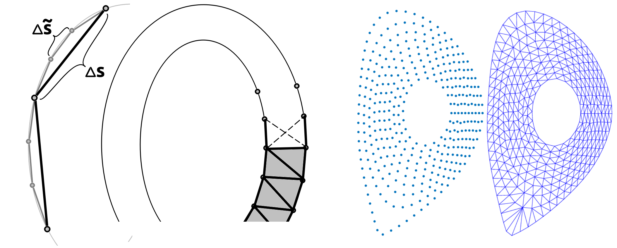
\noindent However, various flux surfaces have different closed-loop lengths and could lead to unevenly spaced first and last grid points on the flux surface. To ensure that the grids are uniform on the flux surface, we redefine the preferred grid spacing using the following scheme: we first generate a high-resolution grid along $s$ with $\Delta \tilde{s} = (\Delta s_{sim}/\mathbb{F}_s),$ \noindent where $\mathbb{F}_s>1$ (see Fig.\ref{fig:Meshing}(a)). We find the total number of grid points for a single loop of the $i$-th flux surface, $\tilde{m}_{\theta i}$ and estimate the required number of grid points as, \begin{eqnarray} m_{\theta i} = \left\lfloor \frac{\tilde{m}_{\theta i}}{\mathbb{F}_s}\right\rceil, \label{eqn:mtheta} \end{eqnarray} \noindent where $\lfloor \cdot \rceil$ stands for the nearest integer. Then the preferred grid points are $(R_{ij},Z_{ij}) = (R_{i\tilde{j}},Z_{i\tilde{j}}),$ where $\tilde{j} = \left\lfloor (j-1) (\tilde{m}_{\theta i}/m_{\theta i}) \right\rfloor + 1,$ and $\lfloor \cdot \rfloor$ is the floor function. Then the distance between the first grid point and the last grid point of the flux surface is \begin{eqnarray} \Delta \tilde{s} \left(\tilde{m}_{\theta i} - \left\lfloor (m_{\theta i}-1) \frac{\tilde{m}_{\theta i}}{m_{\theta i}} \right\rfloor - 1 \right) = \Delta \tilde{s} \left(\left\lfloor \frac{\tilde{m}_{\theta i}}{m_{\theta i}} \right\rfloor - 1 \right) \nonumber \end{eqnarray} and from Eq.~(\ref{eqn:mtheta}), we have \begin{eqnarray} \left( \frac{\tilde{m}_{\theta i}}{\mathbb{F}_s}-1 \right) \leq m_{\theta i} \leq \left( \frac{\tilde{m}_{\theta i}}{\mathbb{F}_s}+1 \right).\nonumber \end{eqnarray}

\noindent Therefore, the error in the spacing between consecutive grid points is $\sim \Delta \tilde{s}$. Note that in $R_{ij}$ and $Z_{ij}$, the dimension of the $j$ index depends on $i$ and hence is inconvenient to store as matrices. Instead, we define an array $(R_\alpha, Z_\alpha) = (R_{ij},Z_{ij}),$ where, $\alpha = g_i + j$ and $g_i = \sum_{k=1}^{i-1} m_{\psi k}$.

\noindent In the case of closed flux surfaces, as in the core, we triangulate the annular region between the two neighbouring flux surfaces. For each annular region, we start from an edge that connects the two different flux surfaces along the outer midplane. Then moving in the counter-clockwise direction we have two different choices for the triangle as shown in Fig.~\ref{fig:Meshing}. We choose the one that has minimal perimeter and continue this process till all the triangles are exhausted in the annular region. The triangles are stored as a triplet of indices $(\alpha,\beta,\gamma)$ which are the labels/indices corresponding to the 3 vertices that constitute the triangle. Now for each annulus between flux surface indexed $i$ and $(i+1)$, the number of triangles that this approach will construct is $(m_{\theta i} + m_{\theta (i+1)})$. Therefore, the total number of triangles that will be formed at the end of the process will be $n_\Delta=(m_\psi-1)(m_{\theta i} + m_{\theta (i+1)}).$