Field lines (numerical integrator)
\noindent For an axisymmetric toroidal system, the poloidal flux function is symmetric in the toroidal direction, i.e., $\psi(R,\zeta,Z) = \psi(R,Z)$ such that $\psi$ is minimum at the magnetic axis, and ${\nabla}\cdot\vec{\mathbf{B}} = 0$ implies the equilibrium magnetic field can be written in an orthonormal coordinate system [see Fig.~\ref{fig:coordinates}] as: \begin{eqnarray} \vec{\mathbf{B}} = \vec{\mathbf{B}}_{Pol} + \vec{\mathbf{B}}_{Tor} \nonumber\\ = \Sigma_{Pol} \; \left( \nabla\psi(R,Z) \times \nabla\zeta \right) + \Sigma_{Tor} \; \left( F_{Pol}(\psi) \; \vec{\mathbf{e}}^\zeta \right), \label{eq:equilibrium} \end{eqnarray}
\noindent where $F_{Pol}(\psi)$ is the poloidal current function, such that $F_{Pol}(\psi)>0$; $\Sigma_{Pol} = sign\left( \vec{\mathbf{B}}_{Pol} \cdot (\nabla \psi \times \nabla\zeta) \right)$, $\Sigma_{Tor} = sign\left( \vec{\mathbf{B}}_{Tor} \cdot \vec{\mathbf{e}}^\zeta \right)$. Let the position vector in Euclidean space be \begin{eqnarray} \vec{\mathbf{X}} = \{ x, y, z \} = \{R \: \cos\zeta, R \: \sin\zeta, Z \} \\ \sigma^1 = R, \; \sigma^2 = \zeta, \sigma^3 = Z. \end{eqnarray} \noindent Therefore, the coordinate tangent vectors and the metric tensors are \begin{eqnarray} \vec{\mathbf{e}}_i &=& \frac{\partial\vec{\mathbf{X}}}{\partial\sigma^i}, \;\; g_{ij} = \frac{\partial\vec{\mathbf{X}}}{\partial\sigma^i} \cdot \frac{\partial\vec{\mathbf{X}}}{\partial\sigma^j} \end{eqnarray}
\noindent By defining contravariant basis vectors $\vec{\mathbf{e}}^R = \nabla R$, $\vec{\mathbf{e}}^\zeta = \nabla \zeta$, $\vec{\mathbf{e}}^Z = \nabla Z$, and $\vec{\mathbf{e}}^i = g^{ij} \; \vec{\mathbf{e}}_j$, the metric component for this orthogonal basis, velocity, and magnetic field can be written as \begin{eqnarray} g_{RR} = 1, \;\; g_{\zeta\zeta} = R^2, \;\; g_{ZZ} = 1, \;\; \text{and} \;\; g_{ij} = 0, \;\; \text{if} \; i\neq j \end{eqnarray} \begin{eqnarray} \vec{\mathbf{v}} \; = \; v^R \vec{\mathbf{e}}_R + v^\zeta \vec{\mathbf{e}}_\zeta + v^Z \vec{\mathbf{e}}_Z \; = \; v_R \vec{\mathbf{e}}^R + v_\zeta \vec{\mathbf{e}}^\zeta + v_Z \vec{\mathbf{e}}^Z \end{eqnarray} \begin{eqnarray} \vec{\mathbf{B}} &=& \tilde{B}^R \; \vec{\mathbf{e}}_R + \tilde{B}^Z \; \vec{\mathbf{e}}_Z + \tilde{B}^\zeta \; \vec{\mathbf{e}}_\zeta = \tilde{B}_R \; \vec{\mathbf{e}}^R + \tilde{B}_Z \; \vec{\mathbf{e}}^Z + (R \; \tilde{B}_\zeta) \; \vec{\mathbf{e}}^\zeta \label{eq:magneticbasis} \end{eqnarray} \noindent Equations ~(\ref{eq:equilibrium}) and ~(\ref{eq:magneticbasis}) provide the components of the magnetic field in cylindrical coordinates as \begin{eqnarray} \tilde{B}_R = -\frac{\Sigma_{Pol}}{\mathcal{J}} \; \frac{\partial \psi} {\partial Z} ; \;\; \tilde{B}_Z = \frac{\Sigma_{Pol}}{\mathcal{J}} \; \frac{\partial \psi} {\partial R} ; \;\; \tilde{B}_\zeta = \Sigma_{Tor}\frac{F(\psi)}{R}, \label{eq:magfiecomp} \end{eqnarray} \noindent where $\mathcal{J}$ is the Jacobian of the transformation, given by $\mathcal{J}=\sqrt{Det[g_{ij}]}$. \noindent The magnitude of the magnetic field is, \begin{eqnarray} B = \sqrt{g^{ij} B_i B_j}= \sqrt{\tilde{B}^2_R + \tilde{B}^2_Z + \tilde{B}^2_\zeta} \end{eqnarray}
\noindent In the presence of an external magnetic field, the plasma has a high degree of anisotropy, with vastly different length and time scales along the magnetic field lines and perpendicular to it. So to maintain the separation of scales and simplify calculations, it is convenient to define a coordinate system that encodes the field line geometry. We build the simulation grids which consider the anisotropy to enable efficient computation. The fields typically vary slowly in the $\parallel$-direction compared to the perpendicular directions. The magnetic field's global structure can be derived by integrating the differential equation of a curve which follows a magnetic field line. The local tangent to the magnetic field $d\mathbf{\mathcal{C}}_\mathbf{B}(s)/ds$, considering $\mathbf{\mathcal{C}}_\mathbf{B}(s)$ to be the trajectory along a magnetic field, can be written as: \begin{eqnarray} \frac{d\mathbf{\mathcal{C}}_\mathbf{B}(s)}{ds}\bigg|_{\text{along}\;\vec {\mathbf{B}}}=\frac{\vec{\mathbf{B}}}{B}=\hat b \label{Eq:Fieldline_vector} \end{eqnarray}
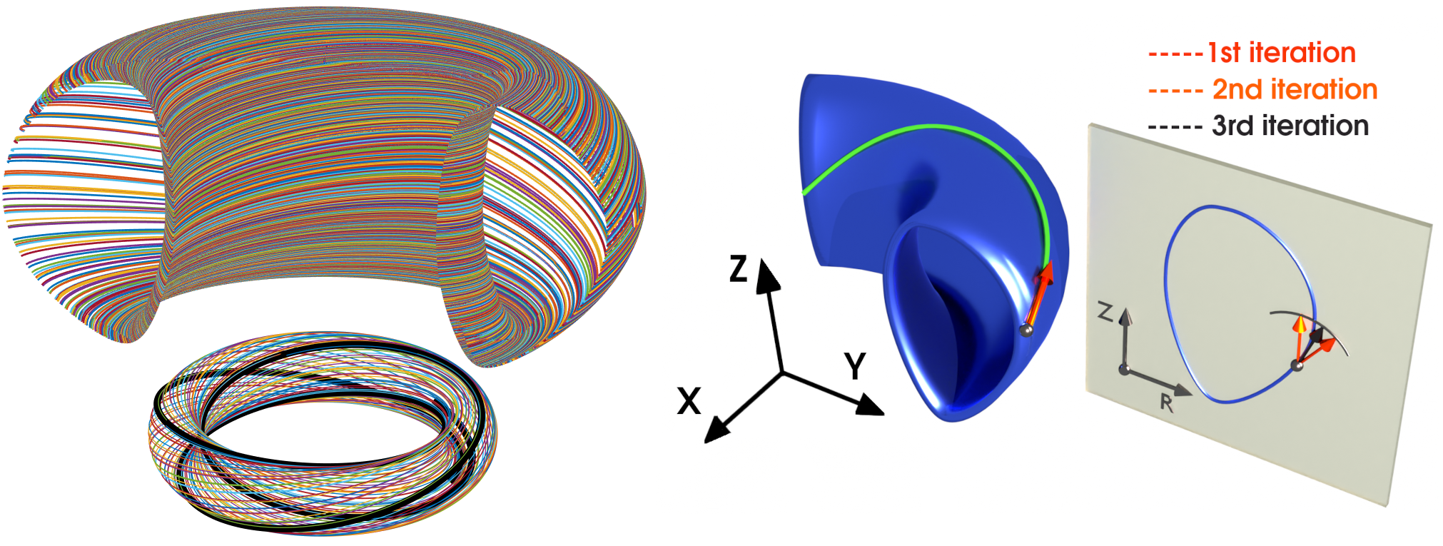
\noindent We parametrize the flux line/curve using its natural length $s$, such that $ds^2 = dx^2+dy^2+dz^2$. Then the flux-line is given by: $\mathbf{\mathcal{C}}_\mathbf{B}(s) = \left\{ x(s), \; y(s), \; z(s) \right\}$. If $\vec{\mathbf{B}}(\mathbf{X})$ is the magnetic field in Euclidean 3d space, i.e. $\mathbf{X}\in \mathbb{R}^3$, then the magnetic flux line is the integral curve corresponding to $\hat b$ and this curve through a point $\mathbf{X}_0$ is given by: \begin{eqnarray} \mathbf{X}(s) = \mathbf{X}_0 + \int_0^s \hat{b}\left(\mathbf{X}(\tilde{s}) \right) \; d\tilde{s} \label{eq:Flux_Line} \end{eqnarray} \noindent The equation above for the flux line can be solved numerically by discretizing $s$ and using \hl{Euler's} method as, \begin{eqnarray} \mathbf{X}(s_i) = \mathbf{X}(s_{i-1}) + \; \Delta s \; \; \hat{b}\left(\mathbf{X}(s_{i-1}) \right) \nonumber \end{eqnarray} \noindent where $\Delta s = (s_i - s_{i-1})$. Figure~\ref{Fig:FieldLines}(a) shows the numerically estimated trajectories for the DIII-D flux profiles using the Euler scheme (and the $\psi$-invariance scheme described in Sec.~\ref{Sec:Psiinvariance}), starting from all grid points of a given flux surface, $\psi=0.28$ at $\zeta=0$. To numerically study the plasma in a tokamak, the computational space is divided into a discrete set of poloidal planes, specified by $\zeta_i = i\; \Delta\zeta$, where $i\in\{1,2,... N_p\}$, $\Delta\zeta = 2\pi/N_p$, and $N_p$ is the number of poloidal planes. Any computation on points in between these poloidal planes, the point is projected onto the nearest poloidal planes along the flux line given by Eq.~(\ref{eq:Flux_Line}). But the estimation of $s$ on the $\zeta_i$'s is non-trivial. If $d\zeta/ds \neq 0$ at all points along the flux line, we can simplify the estimation of projected points by parametrizing the curve using $\zeta$. Therefore, \begin{eqnarray} \frac{d\mathbf{X}}{d\zeta} = \frac{ds}{d\zeta} \; \frac{d\mathbf{X}}{ds} = \frac{ds}{d\zeta} \; \hat{b}, \label{eq:xszeta} \end{eqnarray} \noindent so \st{that} \hl{the} Euler scheme based linear projection operator that projects coordinates onto $\zeta_i$ poloidal plane, $\mathcal{P}_{\zeta_i}$ is given by \begin{eqnarray} \mathcal{P}_{\zeta_i} \mathbf{X} &=& \mathbf{X} + \int_\zeta^{\zeta_i} \; \frac{d\mathbf{X}}{d\zeta} \; d\zeta, \nonumber\\ &\approx& \mathbf{X} + (\zeta_i - \zeta) \; \left. \frac{d\mathbf{X}}{d\zeta}\right|_\zeta \;\; \label{eq:euclideanprojection} \end{eqnarray} \noindent Also, \begin{eqnarray} \hat{b} = \frac{d\mathbf{X}}{ds} = \{ \; B_x/B \; , \; B_y/B \; , \; B_z/B \; \} \nonumber \\ = \{ \; \frac{dR}{ds} \; \cos\zeta - R \sin\zeta \; \frac{d\zeta}{ds} \; , %\nonumber \\ \; \frac{dR}{ds} \; \sin\zeta + R \cos\zeta \; \frac{d\zeta}{ds} \; , %\nonumber \\ \; \frac{dZ}{ds} \; \} \label{eq:UnitProjection} \end{eqnarray} \noindent Comparing the first two components we get, \begin{eqnarray} &\frac{d\zeta}{ds}& = (B_y \; \cos\zeta - B_x \; \sin\zeta )/(RB) \; = \; (\hat{\mathbf{e}}_\zeta . \vec{\mathbf{B}}) / (RB) \; = \; \frac{\tilde{B}_\zeta}{RB}, \nonumber \\ &\frac{dR}{ds}& = (B_x \; \cos\zeta + B_y \; \sin\zeta )/B \; = \; (\hat{\mathbf{e}}_R . \vec{\mathbf{B}}) / B \; = \; \frac{\tilde{B}_R}{B}, \nonumber \\ &\frac{dZ}{ds}& = \frac{\tilde{B}_Z}{B}. \label{Eq:FieldLines} \end{eqnarray}
\noindent Assuming $d\zeta/ds \ne 0$ (i.e. magnetic field is never purely poloidal), we can write $ds/d\zeta = (d\zeta/ds)^{-1}$ and $\Delta s \approx (R \; B / B_\zeta) \Delta\zeta$. Therefore, \begin{eqnarray} R &\rightarrow& R + \Delta s \; \frac{dR}{ds} = R + \Delta\zeta \; \frac{R \; B_R}{\tilde{B}_\zeta} , \nonumber \\ Z &\rightarrow& Z + \Delta s \; \frac{dZ}{ds} = Z + \Delta\zeta \; \frac{R \; B_Z}{\tilde{B}_\zeta} , \nonumber \\ \zeta &\rightarrow& \zeta + \Delta s \; \frac{d\zeta}{ds} = \zeta + \Delta \zeta,\nonumber \\ s &\rightarrow& s + \Delta\zeta \; \frac{R \; B}{\tilde{B}_\zeta}. \label{Eq:FieldLineUpdate} \end{eqnarray}
%%%
Invariance of $\psi$ along the field lines:
\noindent As indicated in the schematic of the flux-surface in Fig.~\ref{Fig:FieldLines}(a), the field line should lie on the same flux surface, {\it i.e.} $\nabla_\parallel \psi = 0$. Conversely, the flux-surface constrains the magnetic field lines. So we need to ensure that the newly estimated point on the discrete flux-line has the same $\psi$ value. We impose this constraint at each update step in Eq.~(\ref{Eq:FieldLineUpdate}) by an iterative projection onto the flux-surface as shown in Fig.~\ref{Fig:FieldLines}(b). We modify the update equation such that if \begin{eqnarray} \alpha = \arctan( \Delta Z / \Delta R ) \;, \;\; \text{and} \;\; r = \sqrt{\Delta R^2 + \Delta Z^2}, \end{eqnarray} then \begin{eqnarray} \Delta R &\rightarrow & r \; \cos(\alpha), \nonumber \\ \Delta Z &\rightarrow & r \; \sin(\alpha), \nonumber \\ \Delta \psi &\rightarrow & \left[ \psi(R+\Delta R,Z+\Delta Z) - \psi(R,Z) \right], \nonumber \\ \Delta \alpha &\rightarrow & sign(\Delta \psi) \; \frac{|\Delta \alpha|}{2}, \;\nonumber \\ \alpha &\rightarrow & \alpha + \Delta \alpha. \label{Eq:UpdateCorrection} \end{eqnarray} \noindent The above iteration is performed with initial $\Delta \alpha = \pi/2$, until $|\Delta\psi|$ is less than a predefined cut-off value. This ensures that the field lines do not deviate by more than the cut-off from the starting $\psi$ at all iterations.